Some more updates on my Political Survey:
(One quick note. I am not a statistician; the procedures I describe below satisfy me intuitively, but I'd be very interested to hear informed criticism of them.)
Analysis so far indicates that only the first two axes in the data are significant. This is of itself a useful and interesting result.
To summarise, the procedure here is to create sample data which is uncorrelated but which has the same marginal distributions (for each statement) as the real data. The eigenvalues of the covariance matrix from the random data set tell us how large an eigenvalue can arise by chance. So we argue that the only eigenvalues from the real data which are significant are those which are significantly larger than the corresponding random-data eigenvalues.
Obviously we'll get different answers for the random-data eigenvalues for each sample random data set we use. So to make the above result robust, we should repeat the random sampling procedure and compute the mean and standard deviation of the random eigenvalues. This is done repeatedly until the mean and standard deviation converge.
My next concern is to determine how well-constrained the eigenvectors are. It's not obvious how best to do this, but what I've done now is to take random subsets of the data -- I've selected, for no very good reason, three-quarters of all responses -- and compute the eigenvectors and eigenvalues of the subsets. This then gives a mean and standard deviation for each eigenvalue and each eigenvector component. The eigenvalues can then be compared directly against the random eigenvalues, as above; we can also inspect the eigenvector components to judge how well-constrained each eigenvector is.
So, the results.
Eigenvalues
Here we plot the random eigenvalues, the eigenvalues obtained from the whole data set, and +/- one standard deviation eigenvalues taken from the three-quarter size subsets (about 250 are sampled to produce these results):
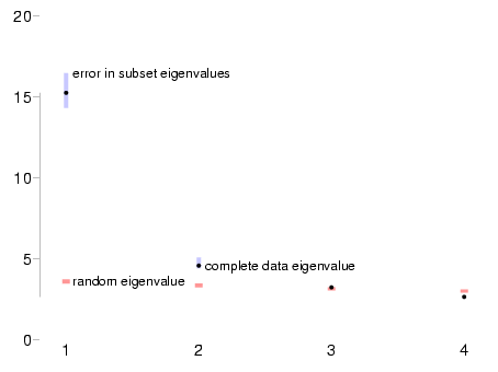
This confirms the statement above: the first two eigenvalues are significant, the first much more than the second; and the standard deviation of the eigenvalues is small, both by comparison with the difference between them -- meaning that we won't confuse eigenvectors 1 and 2 -- and compared the the difference between random and real eigenvalues -- meaning that it's very probable that these eigenvalues do represent real variability in the data.
(One thing I don't understand in this plot is that the eigenvalues derived from the complete data set -- shown by black dots -- don't lie on the mean of the eigenvalues derived from the data subsets. I don't understand why they shouldn't; it's possible that the sampling code hasn't converged properly. I don't think that this is a significant problem, though.)
Eigenvectors
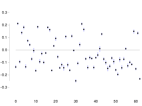
Next we look at the variation in the components of the first two eigenvectors. In these plots, the horizontal axis refers to the statement number, and the vertical axis is the size of this component of the eigenvector. The position of a respondent along this axis is given by the dot-product of their responses with the eigenvector; that is, the sum of the eigenvector components multiplied by the corresponding statement answers. So a large positive value for an eigenvector component means that an `agree' answer to the corresponding statement pushes you towards the positive end of the axis. (You can see the most important statements in the eigenvectors in the existing data report, though these will change slightly when I upload the newer version of the code.)
-
First eigenvector
-
Second eigenvector
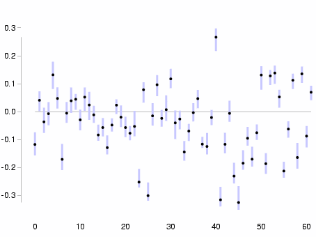
We can see immediately that the first eigenvector is quite well-defined -- the errors in the components are small by comparison to the sizes of the components; and the second eigenvector is poorly defined by comparison, but again the errors are not very large relative to the components.
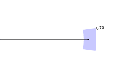
A more intuitive way to look at this is to look at the angles between the subset eigenvectors and the eigenvector derived from the whole data set. So:
-
First eigenvector
-
Second eigenvector
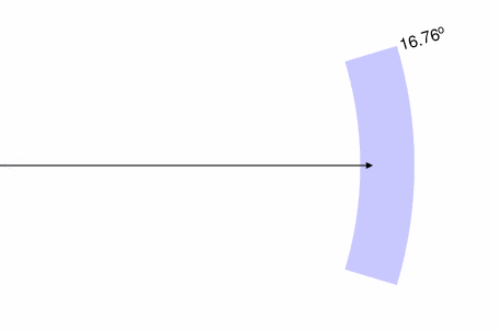
In these plots, the black arrow represents the eigenvector derived from the whole data set. The blue region shows (a) the variation in the eigenvalue, as a variation along the length of the vector; (b) the variation in the direction of the eigenvector itself. The first eigenvector is well-constrained, varying on the order of 6.7° depending on which three-quarters of the data we use to derive it; the second eigenvector is more poorly defined, varying by around 16.76°.
Note that in both cases the variation in direction is much less than 45°, which suggests that we are not confusing the first two eigenvectors with others.
Hence, it seems reasonable to stick the results from these calculations into the results script and start displaying where respondents fall in the two-dimensional space defined by these eigenvectors. I'll try to do that later this weekend.